Causal Inference & Experimentation

A field guide to answering "did it work?" — from randomized experiments to the designs you reach for when you can't randomize. Every method below is implemented from scratch in an open-source companion repo where estimators are graded against known true effects.

Why any of this matters

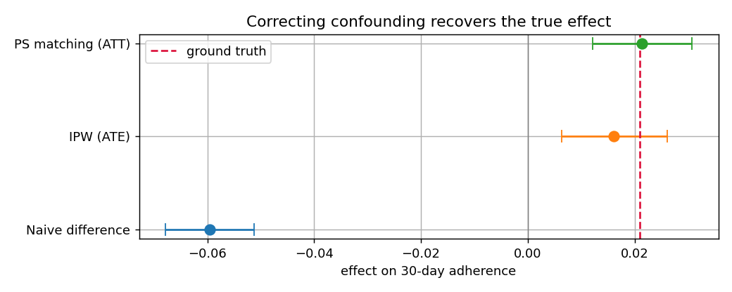
A healthcare outreach program truly improved medication adherence by +2.1 points. But care coordinators enrolled the sickest patients — so the naive comparison of enrolled vs. not-enrolled showed −6.0 points: a genuinely helpful program looked harmful. Correlation didn't just miss the causal effect; it flipped its sign. Every method on this page is a strategy for not making that mistake.

Chart showing the naive estimate with the wrong sign, while IPW and matching estimates recover the true effect
The naive comparison (top) gets the sign wrong; propensity-based corrections recover the true effect (red dashed line). From case study 3 in the companion repo.

Part 1 — Causal Foundations

Potential outcomes

A causal effect compares what a unit's outcome would be with treatment, Y(1), versus without, Y(0). Each unit reveals only one of the two — the fundamental problem of causal inference. Every method here is a strategy for estimating averages of effects despite half of each comparison being forever missing.

Selection bias

The naive contrast equals the causal effect plus a bias term: how the treated would have differed even without treatment. Randomization is the one design that deletes this term outright — which is why experiments are the default and everything else is the fallback.

Estimands: ATE, ATT, LATE

Decide what you're estimating before how: the average effect for everyone (ATE), for the treated (ATT), for units an instrument can move (LATE), or at a threshold (RDD). Under heterogeneous effects these are different numbers for the same program — say which one you're reporting, always.

Confounders, mediators, colliders

Causal graphs (DAGs) give the adjustment rule: control for confounders (common causes), never for mediators (the mechanism) if you want the total effect, and never for colliders (common consequences) — conditioning on a collider manufactures bias. "Control for everything" is not a safe default.

Part 2 — Main Causal Designs & Models

When you can't randomize, each design buys identification with a different assumption. Report the estimate next to the diagnostics that interrogate exactly that assumption.

Difference-in-differences

Compare the treated group's before–after change with an untreated group's change; stable group differences cancel out.

Key assumption Parallel trends — probeable with pre-period data.

Use when A policy or launch hits one group at a known time.

Synthetic control

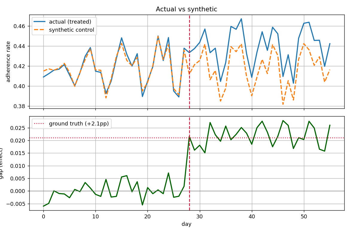
Build a weighted blend of untreated markets that tracks the treated market pre-launch; the post-launch gap is the effect. Inference by placebo permutation. The engine behind geo experiments.

Key assumption Pre-period fit predicts the counterfactual.

Use when Rollouts are market-by-market and users interfere.

Instrumental variables (2SLS)

A variable that nudges treatment but touches the outcome only through treatment (a randomized encouragement letter, distance to a clinic) identifies the effect for compliers — the LATE — even with unobserved confounding.

Key assumption Exclusion (untestable); relevance is testable — report the first-stage F.

Use when Take-up is self-selected but the nudge was (as-good-as) random.

Regression discontinuity

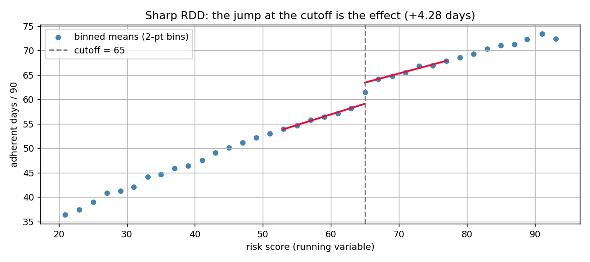
When a threshold rule assigns treatment (risk score ≥ 65 → auto-enroll), units just above and below the cutoff are locally comparable; the jump in the outcome at the cutoff is the effect.

Key assumption No precise manipulation of the score; check placebos, bandwidths, density.

Use when Eligibility is score- or cutoff-based. Estimate is local to the threshold.

Propensity scores: IPW & matching

Model the probability of treatment given observed covariates, then reweight (IPW) or match units to mimic a randomized comparison. Balance and overlap diagnostics are most of the job.

Key assumption No unmeasured confounding — untestable.

Use when Selection runs through covariates you actually observe.

Doubly robust (AIPW)

Combine an outcome model with propensity weights: consistent if either model is right. The same construction underlies double/debiased machine learning.

Key assumption Same as propensity methods — but one wrong nuisance model is survivable.

Use when You're adjusting on observables and want model-misspecification insurance.

Sensitivity analysis (E-values)

"No unmeasured confounding" can't be verified — only quantified. The E-value is the minimum strength an unmeasured confounder would need, with both treatment and outcome, to fully explain away your estimate.

Use when Always — next to every observational estimate you report.
Synthetic control chart: actual vs synthetic series and the post-launch gap
Synthetic control in action: the weighted donor blend tracks the treated markets pre-launch; the post-launch gap recovers the true +2.1pp effect. From case study 2.

Part 3 — Panel & Longitudinal Models

Repeated measurement of the same units is a design resource of its own: anything stable about a unit — measured or not — cancels out of within-unit change. That removes a class of confounding no covariate list can.

Fixed & random effects

Fixed effects (the within estimator) demeans each unit's data, removing all stable confounding; identification comes from within-unit change. Random effects is more efficient but assumes the unit effect is uncorrelated with the regressors; the Hausman test arbitrates. DiD is FE's two-period special case.

Caveat FE can't fix time-varying confounding, and can't estimate time-constant predictors.

Cross-lagged panel models

Two processes co-evolve — engagement and study time, strain and health. Which leads? Regress each wave on the previous wave of both. The classic caveat (RI-CLPM): without modeling stable trait differences, cross-lags mix within-person influence with "high-x people are high-y people".

Use when The question is temporal precedence, not a single treatment effect.

Latent growth curves

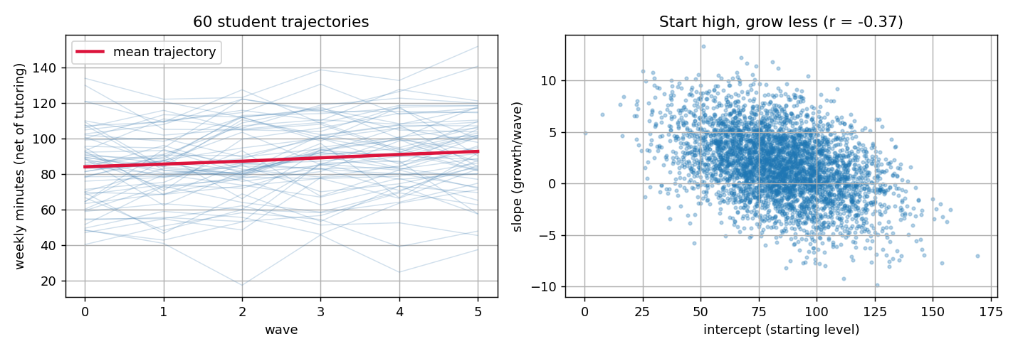
Give every unit its own trajectory (intercept + slope) and model the distribution: average growth, how much growth varies, and whether units that start high grow faster. Individual change becomes the estimand instead of a nuisance.

Use when Development over time is itself the outcome — learning, adherence, careers.

SEM & latent variables

Structural equation models chain regressions into path models and add measurement models: latent constructs measured by multiple indicators, correcting the attenuation that measurement error causes in any regression. Growth curves and RI-CLPMs are special cases. The causal content still comes from the assumed graph — not the fitting machinery.

Marginal structural models

With time-varying treatment, a time-varying confounder can also be a mediator — plain regression and FE both fail. The g-methods (IPW over treatment histories, g-computation) are the standard solution from epidemiology.

Use when Treatment and confounders feed back on each other over time.

Latent growth curve figures: individual student trajectories with the mean trajectory, and the intercept-slope scatterplot
Latent growth curves on six waves of student data: individual trajectories around the mean (left), and the recovered intercept–slope correlation — students who start high grow less (right). From case study 4.

Part 4 — Experimentation

When you can randomize, the assumptions become about execution — and execution is checkable. A trustworthy A/B pipeline is design, integrity, then analysis, in that order.

Power analysis & MDE

Size the test before collecting data, for the smallest effect that would change the ship decision — not the effect you hope for. Underpowered tests are the most common experimentation failure.

Randomization & bucketing

Salted-hash bucketing: hash (salt, user id) to a variant. Deterministic — same user, same variant, no storage — and different salts give independent assignments, which is what lets many experiments overlap safely. Geo and switchback designs handle interference.

Integrity: SRM & A/A tests

Sample-ratio mismatch (a chi-square on the observed split) means assignment or logging is broken — results must not be read. A/A tests validate the whole pipeline: null experiments should produce uniform p-values. Check integrity before metrics, always.

Variance reduction (CUPED)

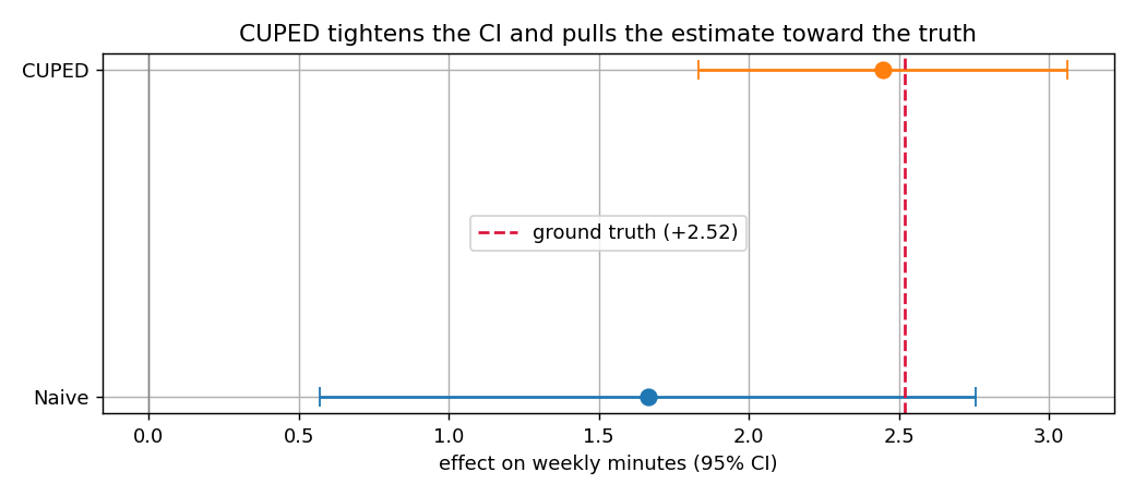
Subtract the part of the outcome predictable from pre-experiment behavior. Same effect estimate, much tighter interval — routinely worth 2–3× the effective sample size.

Ratio metrics & clustering

CTR-style metrics are ratios of correlated within-user events — treating each event as independent understates the variance (delta method fixes it). Same trap when analysis is finer than randomization: cluster-robust SEs on the assignment unit.

Sequential testing

Stakeholders will peek daily; repeatedly checking a fixed-horizon p-value inflates false positives badly. Always-valid p-values (mSPRT) and confidence sequences keep the guarantee under continuous monitoring and optional stopping.

Multiple testing

A metric scorecard is many tests read together: with enough null metrics, something "wins" by chance. Benjamini–Hochberg controls the false-discovery rate for exploratory metrics; Bonferroni protects a short pre-registered guardrail list.

Bayesian readouts

Ship decisions ask "what's the probability treatment is better, and what do we lose if we're wrong?" — P(better) and expected loss, the quantities a launch review actually uses.

CUPED vs naive t-test confidence intervals against the known true effect
CUPED cuts the confidence interval roughly in half at the same sample size — both intervals cover the known truth (red dashed line). From case study 1.

Part 5 — Which Design, When

Ordered by how much the conclusion leans on untestable assumptions. When a choice exists, move up the ladder.

SituationDesignKey assumption to defend
You can randomize usersA/B testExecution: no SRM, no interference
Users interfere (marketplaces, pricing)Switchback / cluster randomizationEffects don't bleed across time blocks
Rollout is market-by-marketGeo experiment + synthetic controlPre-period fit predicts the counterfactual
Policy hit one group at a known timeDifference-in-differencesParallel trends
Assignment was nudged by something excludableInstrumental variablesExclusion restriction; strong first stage
A threshold rule assigns treatmentRegression discontinuityNo precise manipulation at the cutoff
Same units measured repeatedlyFixed effects / DiDNo time-varying confounding
Trajectories of change are the questionLatent growth curvesGrowth-shape specification
Which of two processes leadsCross-lagged panel (RI-CLPM)Stable traits modeled, lags well-specified
Only observed covariates separate groupsPropensity methods / AIPWNo unmeasured confounding + report E-values

Part 6 — Case Studies & Code

The companion repo, experimentation-hub, implements everything above from scratch in pure numpy/pandas — no black boxes — on synthetic data with configured true effects, so every estimator is graded on whether it recovers the truth. Five executed case-study notebooks walk through the design choices:

Case studyQuestionTruthEstimate
01 — Classic A/B (education)Adaptive hints → study minutes+2.52 min+2.45 (CUPED), CI [+1.83, +3.06]
02 — Geo experiment (healthcare)Outreach → adherence+2.1pp+2.2pp (synthetic control, placebo p < 0.01)
03 — Quasi-experiment (healthcare)Same, self-selected enrollment+2.1ppnaive −6.0pp (!) → +2.1pp matched
04 — Panel & growth (education)Tutoring → study minutes+6.0 minpooled OLS +23.5 (!) → FE +6.0
05 — IV & RDD (healthcare)Enrollment → adherent days+6.0 daysOLS +13.0 (!) → 2SLS +5.9
Regression discontinuity plot: binned means of the outcome by risk score, with fitted lines on each side of the cutoff showing the jump
Sharp regression discontinuity at a risk-score cutoff: the jump between the fitted lines is the treatment effect (+4.3 estimated vs. +4.0 true). From case study 5.

All code, notebooks, methodology notes, and 31 known-truth tests are open source.

View on GitHub