Optimization Methods

A field guide to making the best decision a model can defend: which plants to open, which route to drive, which schedule to run. From exact methods that come with proofs to metaheuristics and quantum annealing that trade proofs for reach. Every family below has a flagship algorithm implemented from scratch in an open-source companion repo, graded against known optima.

Why any of this matters

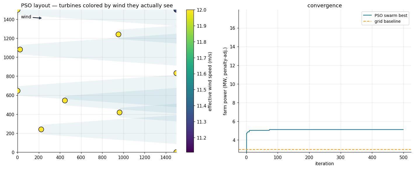
Ten wind turbines placed on a sensible engineering grid produce 2.98 MW, because each turbine's wake robs the ones behind it of wind. A particle swarm searching the same site found a staggered layout producing 5.10 MW: 71% more power from identical hardware, within 1.6% of the physical ceiling, purely by rearranging positions. Optimization is the discipline of finding those arrangements on purpose, and of knowing how far from the best possible answer you might still be.

Wind farm layout found by particle swarm optimization, with wake cones and turbines colored by the wind speed they receive, next to the convergence curve beating the grid baseline
The swarm pushes turbines upwind and staggers the rest so wake cones slide between rows (left); convergence vs. the grid baseline (right). From case study 3 in the companion repo.

Part 1: Foundations

Anatomy of a problem

Every optimization problem has the same skeleton: decision variables (what you control), an objective (what you want more or less of), and constraints (what reality permits). The entire zoo of methods is about one question: what structure do these three have (linear, convex, discrete, noisy, black-box), and what can be exploited?

Convexity: the great divide

In a convex problem, any local optimum is global, and polynomial-time algorithms exist that terminate with a certificate of optimality. Non-convex landscapes have many basins, and no general method can promise the best one. The first diagnostic question for any new problem: is there convex structure to exploit, or can the problem be reformulated so there is?

The combinatorial wall

Add yes/no decisions to a linear program and it becomes NP-hard. A 30-stop delivery route has more possible tours than atoms in the observable universe; a modest job-shop has ~1033 schedules. Past some scale, proving optimality is hopeless, which is the economic justification for every heuristic on this page.

Certificates vs. "good enough"

Exact methods return the answer plus a proof (a bound on money left on the table). Heuristics return an answer and silence. The professional discipline for heuristics: validate the engine on instances with known optima, then grade real runs against provable bounds and honest baselines such as greedy or random-with-equal-budget.

No free lunch

Averaged over all possible problems, every optimizer performs identically. That is a theorem, not a slogan. A method only wins by exploiting structure: linearity, smoothness, decomposability, locality of good moves. The craft is matching method to structure, never defending a favorite hammer.

Part 2: Exact Methods (Mathematical Programming)

Declare the algebra (variables, linear or convex objective, constraints) and a solver returns the optimum with a certificate. When your problem fits this box, nothing else on this page should be your first choice.

Linear programming (LP)

Linear objective, linear constraints, continuous variables. The simplex method walks vertex to vertex of the feasible polytope, always improving; interior-point methods cut through the middle. Duality yields shadow prices, the marginal value of each constraint, often worth more than the solution itself.

Use when Allocating scarce resources with linear trade-offs. Scale is effectively unlimited.

Industries Production planning, blending (refineries, feed), ad budget allocation, transportation.

Mixed-integer LP (MILP)

LP plus integer variables for yes/no and how-many decisions. Branch & bound solves LP relaxations, branches on fractional integers, and prunes subtrees whose bound can't beat the incumbent; branch & cut adds cutting planes. NP-hard, yet modern solvers routinely crack thousands of binaries.

Use when Discrete decisions with linear structure and a need for provable quality.

Industries Facility location, crew & fleet scheduling (airlines), power unit commitment, network design.

Quadratic & conic (QP, SOCP, SDP)

Convex quadratic objectives and cone constraints keep the certificate while adding curvature: portfolio variance, least squares with constraints, robust counterparts. Interior-point methods solve them in polynomial time.

Use when Risk or squared-error terms enter a convex objective.

Industries Portfolio construction, energy dispatch, control, structural design.

Nonlinear programming (NLP)

Smooth nonlinear objectives or constraints. SQP and interior-point methods converge to local optima; global only under convexity. Good initial points and multistart are part of the method, not an afterthought.

Use when Physics or chemistry enters the constraints and gradients exist.

Industries Chemical process design, optimal power flow, trajectory optimization.

Constraint programming (CP)

Feasibility-first search with domain propagation: each constraint actively prunes the possible values of its variables. Shines where constraints are rich and logical (precedences, all-different, calendars) and the objective is thin.

Use when "Find any legal schedule" is most of the battle.

Industries Timetabling, rostering, configuration, manufacturing sequencing.

Dynamic programming (DP)

When decisions decompose over stages with optimal substructure, solve each subproblem once and reuse it: shortest paths, inventory policies, Held–Karp for TSP. Exact, but the state space explodes exponentially with dimension (the "curse of dimensionality").

Use when Sequential decisions with a compact state.

Industries Inventory control, routing engines, revenue management, RL foundations.

Specialized combinatorial algorithms

Max-flow/min-cut, shortest paths, assignment (Hungarian algorithm), matching, spanning trees: polynomial-time exact algorithms for specific structures. Always check whether your problem is one of these in disguise before reaching for anything heavier.

Use when The problem maps to a known graph structure.

Industries Logistics networks, matching markets (riders–drivers, ads), telecom routing.
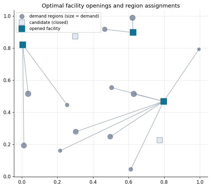
Map of demand regions connected to the facilities branch and bound chose to open, with closed candidates shown in gray
Branch & bound on a facility-location MILP with a capex budget: 3 of 5 candidate facilities opened, every region served by its cheapest open facility, certified optimal in 4 nodes against 31 enumerated subsets. From case study 1.

Part 3: Continuous & Black-Box Methods

Between the algebra of exact methods and the population games of metaheuristics sits continuous search: follow the gradient when you have one, model the landscape when you don't.

Gradient descent & friends

Step downhill along the negative gradient. With momentum, adaptive step sizes (Adam), and stochastic mini-batches, this is the workhorse of machine learning: cheap per step, scales to billions of parameters, converges to local optima only.

Use when Smooth objective, gradients available (autodiff), huge dimension.

Newton & quasi-Newton

Use curvature, not just slope: Newton's method rescales steps by the Hessian; BFGS/L-BFGS approximate it from gradient history. Far fewer iterations than plain descent on smooth, moderate-dimension problems, and the default for classical statistical fitting.

Use when Smooth objectives up to ~104 dimensions where per-step cost is affordable.

Derivative-free local search

Nelder–Mead crawls a simplex of points downhill using only function values, with no gradients and few assumptions. Reliable for cheap, low-dimensional, smooth-ish problems; degrades quickly past ~10 dimensions.

Use when Tuning a handful of parameters of a simulation or legacy code.

Bayesian optimization

When each evaluation costs hours or dollars, spend them wisely: fit a probabilistic surrogate (a Gaussian process) to the evaluations so far and pick the next point by expected improvement, balancing exploring uncertain regions against exploiting promising ones.

Use when Expensive black-box evaluations, small budgets, ≲20 dimensions.

Industries ML hyperparameters, lab & process experiments, chip design, drug formulation.

CMA-ES & differential evolution

Population methods purpose-built for rugged continuous landscapes. CMA-ES adapts a full covariance of its sampling distribution and is the gold standard for hard black-box continuous problems; differential evolution mutates by vector differences and is a robust, nearly tuning-free default.

Use when Non-convex continuous problems where gradients are unavailable or lie.

Part 4: Metaheuristics

General-purpose search strategies for problems that are discrete, non-convex, black-box, or all three. No certificates, so the discipline is in the baselines. Two families: trajectory methods perturb one solution; population methods evolve many and share information.

Simulated annealing

A random walk that always accepts improvements and accepts worsening moves with probability e−ΔE/T, where the temperature T cools over time: roam early, commit late. Simple, robust, and one real design decision: the neighborhood move, where all the domain knowledge lives.

Use when Discrete states, computable objective, good "local move" structure.

Industries Vehicle routing, chip floorplanning, cell-tower placement, timetabling.

Tabu search

Greedy local search plus memory: recently-made moves become tabu, so the search can't immediately undo them and is forced out of local optima deterministically. Long-term memory adds diversification. Often the strongest single-solution method on scheduling and routing.

Use when A strong local search exists but keeps getting trapped.

Iterated local search & VNS

Run local search to a dead end, perturb the result, then run again, keeping the better endpoint (ILS). Variable neighborhood search systematically switches between neighborhood structures when one stalls. Deceptively simple; frequently state-of-the-art.

Use when You already have a decent local search and want a principled restart strategy.

Genetic algorithms

Evolve a population under selection pressure: tournament selection, crossover that recombines building blocks of parents, mutation for diversity, elitism so the best survive. The encoding is where the intelligence lives: a good one makes every genome feasible by construction.

Use when Solutions have meaningful parts worth recombining.

Industries Job-shop scheduling, crew rostering, antenna & structure design, feature selection.

Particle swarm optimization

Particles fly through continuous space pulled by inertia, their own best find (memory), and the swarm's best (social attraction). Information spreads instantly, so one particle's discovery redirects the swarm. The result is fast convergence without gradients, and premature convergence as the known failure mode.

Use when Continuous non-convex problems with cheap evaluations.

Industries Wind-farm & solar layout, engineering design, controller tuning.

Ant colony optimization

Artificial ants build solutions edge by edge, biased by pheromone laid on edges that appeared in good solutions; pheromone evaporates, so bad habits fade. A natural fit for problems whose solutions are paths through a graph.

Use when Constructive, graph-structured problems such as routing and sequencing.

Industries Logistics, telecom packet routing, assembly sequencing.

Matheuristics & hybrids

The pragmatic frontier: metaheuristics that call exact solvers as subroutines, such as large-neighborhood search that destroys part of a solution and re-optimizes it as a MILP, or a GA whose fitness function prices candidates with an LP. Often beats either paradigm alone.

Use when The problem has an exactly-solvable core inside a messy shell.

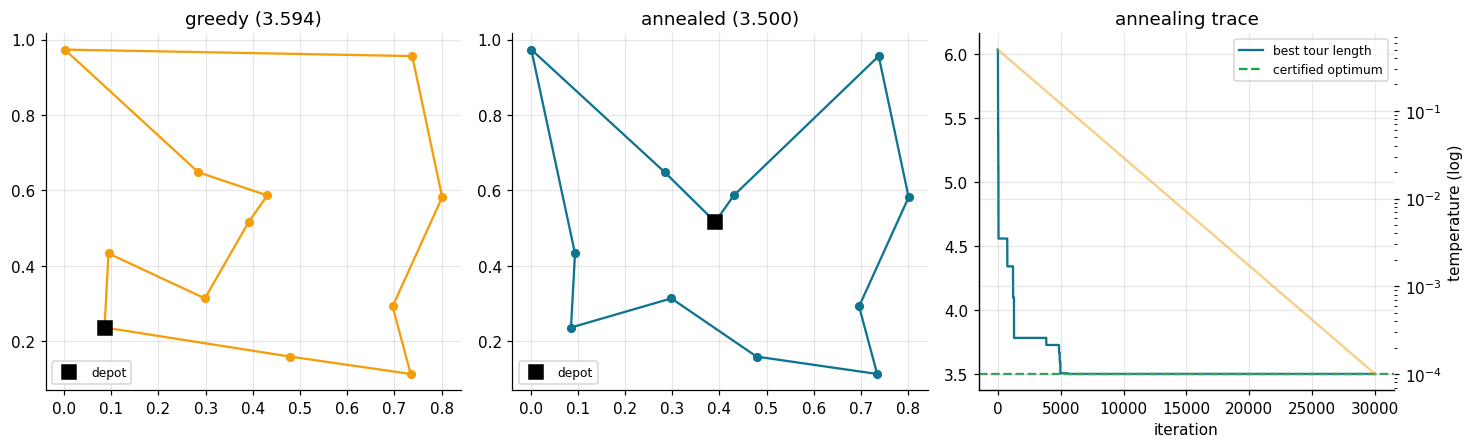
Greedy delivery route with crossing edges, the annealed route without crossings, and the annealing trace converging to the certified optimum
Simulated annealing on a 12-stop delivery route: the greedy route crosses itself (left), annealing uncrosses it and lands exactly on the Held–Karp-certified optimum (center, right). From case study 2.

Part 5: Optimization Under Uncertainty

Real inputs like demand, prices, and travel times are forecasts, not facts. Optimizing as if the point forecast were true systematically overfits to it; these frameworks make the uncertainty part of the model.

Stochastic programming

Optimize expected cost over a tree of scenarios, distinguishing here-and-now decisions (made before uncertainty resolves) from recourse decisions (made after). The value of the stochastic solution measures what point-forecast planning would have cost you.

Use when Distributions are estimable and recourse exists.

Industries Supply planning, energy trading, capacity expansion.

Robust optimization

Optimize against the worst case within an uncertainty set, with no probabilities required. Conservative by design, tractable via convex reformulation, and the right frame when a single bad realization is unacceptable.

Use when Distributions are unknown but bounds are credible; downside is catastrophic.

Industries Network capacity, inventory safety stock, engineering tolerance design.

Chance constraints

Require constraints to hold with probability at least 1−ε: "meet demand 98% of days", "grid stays within limits 99.9% of hours". Sits between expectation and worst case, and maps directly to the service-level language operations already speaks.

Use when Occasional violation is tolerable and priced.

Industries Power systems reliability, service-level logistics, finance risk limits.

Part 6: Quantum & Physics-Inspired Annealing

A different bet: instead of a cleverer algorithm, a different physical substrate. Encode the problem as energy; let a physical (or simulated-physical) system relax to its ground state.

QUBO: the lingua franca

Annealers accept exactly one input: minimize x'Qx over binary x (equivalently, an Ising spin model). Using them is an exercise in formulation: constraints become quadratic penalties in Q, and penalty weights are real modeling decisions with a classic failure mode: too weak and the "constraint" silently stops binding.

Use when The problem is naturally binary-quadratic: selection, partitioning, assignment.

Quantum annealing

Hardware (D-Wave and kin) prepares qubits in superposition and slowly morphs the system toward the problem Hamiltonian; quantum tunneling can pass through thin energy barriers that thermal methods must climb over. Thousands of physical qubits exist today; limited connectivity and noise mean embedding and formulation dominate practice.

Status Real hardware, real workloads, but no demonstrated practical advantage over tuned classical methods yet.

Simulated quantum annealing

The standard classical simulation of the quantum process: path-integral Monte Carlo runs P coupled replicas of the system whose coupling strengthens as the simulated transverse field anneals away, sampling the same distribution the hardware explores physically. A respectable QUBO heuristic in its own right, and the benchmark quantum hardware has to beat.

Use when You want annealing-style search on QUBOs today, on ordinary CPUs.

QAOA & digital annealers

QAOA is the gate-model cousin: shallow parameterized quantum circuits tuned by a classical outer loop, still research-stage. Digital annealers (specialized silicon for Ising problems) are quantum-inspired hardware shipping now. The QUBO formulation skills transfer across all of them unchanged.

Industries piloting Portfolio construction, logistics, molecular conformation, scheduling.

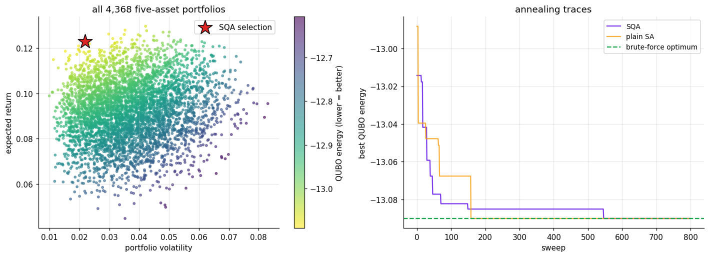
Scatter of all five-asset portfolios by risk and return colored by QUBO energy with the SQA selection starred, next to SQA and SA annealing traces reaching the brute-force optimum
Portfolio selection as a QUBO: among all 4,368 five-asset portfolios (left), simulated quantum annealing lands on the brute-force-certified optimum (star); annealing traces for SQA and classical SA (right). From case study 5.

Part 7: Which Method, When

Two questions sort most real cases. Is there linear or convex structure to exploit? If yes, go exact, because certificates are valuable and modern solvers are fast. If not, what evaluation budget can a search method spend, and what baseline will you grade it against?

Problem looks like…Reach forCertificate?
Linear, continuousLP (simplex / interior point)Yes
Linear + yes/no decisions, moderate scaleMILP (branch & bound / cut)Yes
Convex with curvature (risk, squared error)QP / SOCP (interior point)Yes
Matches a known graph structureDedicated algorithm (flow, matching, DP)Yes
Rich logical constraints, scheduling flavorConstraint programmingFeasibility
Smooth nonlinear, local optimum acceptableNLP (SQP / L-BFGS, multistart)Local only
Discrete, huge, deadline-boundSA / tabu / GA / ACO + bounds & baselinesNo
Continuous black-box, cheap evaluationsPSO / differential evolution / CMA-ESNo
Continuous black-box, expensive evaluationsBayesian optimizationNo
Inputs are forecasts, not factsStochastic / robust programmingModel-relative
Binary-quadratic; exploring new hardwareQUBO + annealer (or SQA today)No

Part 8: Case Studies & Code

The companion repo, optimization-hub, implements a flagship algorithm from each family from scratch in numpy, with no solver libraries and no black boxes, and grades every one against an independently computed optimum: exhaustive enumeration, exact dynamic programming, or vertex search. Five executed notebooks, each a scaled-down industrial decision:

Case studyAlgorithmGround truthResult
01. Supply chain (manufacturing)Simplex + branch & boundVertex / subset enumerationCertified optimum, 4 nodes vs 31 subsets
02. Delivery routing (logistics)Simulated annealing, 2-optHeld–Karp exact DPExact optimum on 12 stops; −14% vs greedy on 30
03. Wind-farm layout (energy)Particle swarmBenchmark functions + baselines2.98 → 5.10 MW vs grid; 1.6% from ceiling
04. Job-shop scheduling (manufacturing)Genetic algorithm, POXAll 1,680 schedules; lower boundExact on 3×3; within 6.5% of bound on 8×5
05. Portfolio selection (finance)Simulated quantum annealingAll 216 bitstringsGround state found; penalty failure mode shown
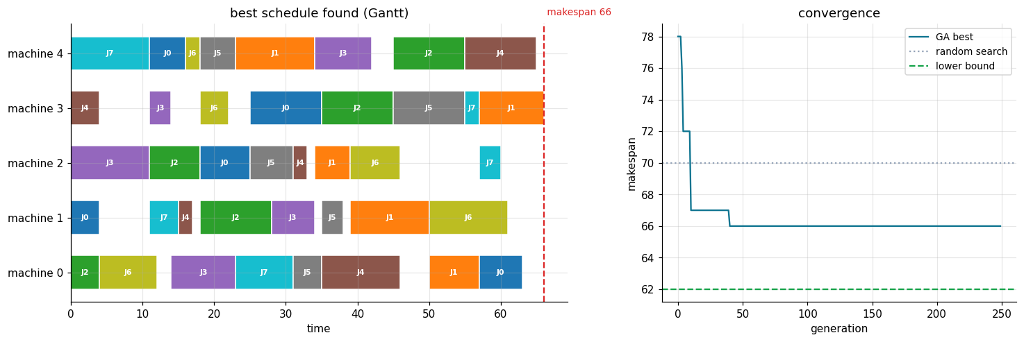
Gantt chart of the best job-shop schedule found by the genetic algorithm, next to the convergence curve approaching the provable lower bound and beating random search
The genetic algorithm's best 8-job × 5-machine schedule as a Gantt chart (left); convergence toward the provable lower bound, beating equal-budget random search (right). From case study 4.

All code, five executed notebooks, the methodology guide, and 15 known-truth tests are open source.

View on GitHub